Sign
The domain contains seven values, from “nothing” to “anything”. Joining 0 and >0 gives ≥0.
A static analyzer reads your program and establishes properties of its executions, without running any. Once it says a check always holds, people stop looking at that line. An error in the analyzer can invalidate that conclusion.
Voblint addresses this problem through a soundness proof in Isabelle/HOL, from source semantics to analyzer verdicts. The result holds whenever the solver finishes. The analyzer in the playground runs the code Isabelle generated from those same definitions. This page explains the analyzer, its results, and what the proofs do and do not cover.
 Isabelle/HOL
 Goblint
 OCaml
 WebAssembly
Analyzer output
Take the program below. It sets k to 10 and divides 100 by it, then
divides 100 by an arbitrary integer d, and finally asks whether
q is positive. It also has a branch that no run can enter. Voblint analyzes
it without running it. It checks every division and remainder for a zero divisor on
its own, without being asked. Any other condition you want checked, you write as a
__voblint_check.
Your program
fun main() {
  k = 10;
  q = 100 / k;
  d = __voblint_nondet_int();
  y = 100 / d;
  __voblint_check(0 < q);
  if (k < 0) {
    __voblint_check(q == 0);
  }
}
Settings
 Voblint
never runs
your program
WARNING possible division by zero: 100 / d
PROVED 0 < q, where q = [10, 10]
DEAD q == 0 sits where no run arrives
At the proved check, the whole state:
k = [10, 10] · q = [10, 10] ·
d = ⊤ · y = ⊤
Three of these rows are claims about every run, and each has a theorem behind it.
PROVED means that whenever a run reaches the check, the condition holds
there
(run_voblint_check_sound).
It does not say that any run gets there. DEAD says that no run reaches
the line
(run_voblint_dead_check_unreached).
The warning works the other way round. A warning means the analysis could not rule out a zero divisor.
The theorem concerns program points with no warning. No run reaching such a point divides by zero in an expression on an outgoing graph edge
(run_voblint_arithmetic_safe).
All three theorems assume that the analyzer's solver finished on this program. The
last row, the whole state at the check, has no theorem. It is the state the analysis
computed, printed as text, and nothing proves that the text says what the state means.
--analysis interval and the default settings. The divisor
warning needs no annotation; the two checks are the program's own. Inside the branch
under k < 0 nothing else would be reported either. Even a division by
zero written there would stay silent, because no run performs it.
Run it ↗
Soundness
Analyzers are programs, and programs have bugs. Many of them make the analyzer too
cautious. An affected analyzer answers UNKNOWN where it could have said more. That costs
precision, but the answer is still right. An unsound analyzer can report PROVED for a check violated by real executions, or DEAD for code that does run, and nobody looks at that line again.
Goblint, a mature analyzer for C, files these bugs under their own label. Below is one of them, reported in issue #1156 and fixed by pull request #1161, replayed with the verdict it got wrong. The notes in the margins are the analyzer's state at each line; the next two sections explain them, and the one after says what a machine-checked proof rules out.
A real bug, replayed
goblint/analyzer #1161: Congruences: Make % sound by restricting cases where we return a constant
#1156
In C, integer division truncates toward zero, so a remainder takes the sign of its dividend. For a negative odd c the result of c % 2 is −1. Goblint's congruence domain describes c as 1+2ℤ, the set of all odd integers, and it evaluated c % 2 to the constant 1 for every such c, regardless of sign. In the program below, c is −5 or −7, so Goblint reported that c % 2 == 1 succeeds, although every run violates it. The program involves no wrap-around, only signed arithmetic, so it means the same thing in VIMP. The dot follows one real run, with top ≠ 0.
Goblint, before the fix
main() {
  int top;
  int c = -5;c = −5
  if (top) {
    c = -7;−5 ⊔ −7 = 1+2ℤ
  }
  ↳ 1+2ℤ % 2 = 1  ✗ every run gives −1
  __goblint_check(c % 2 == 1);✗ will succeed
  __goblint_check(c % 2 == -1);not documented
}
The first verdict is wrong. The check fails in every run. Issue #1156 does not record Goblint's verdict on the second check.
Voblint, congruence only
fun main() {
  top = __voblint_nondet_int();
  c = -5;c = −5
  if (top) {
    c = -7;−5 ⊔ −7 = 1+2ℤ
  }
  ↳ 1+2ℤ % 2 = 1+2ℤ  ✓ holds −1 and 1 both
  __voblint_check(c % 2 == 1);? UNKNOWN
  __voblint_check(c % 2 == -1);? UNKNOWN
}
Neither check is decided, and neither verdict is wrong. With the same domain and the same program, Voblint cannot produce the answers shown on the left.
c = −5top ≠ 0, so c = −7c % 2 = −1c % 2 == 1 is falsec % 2 == -1 is true37-congruence/14-negative.c, with that test's flags --enable ana.int.congruence --set sem.int.signed_overflow assume_none. The fix returns the constant result of % only when the remainder is zero, when the dividend is already a single value, or when the type is unsigned. A signed c that is only known to be odd now yields the class 1+2ℤ. Both analyzers run the congruence domain and arrive at this class. The difference is that Voblint's operation is proved sound (congruence_mod_sound), so the wrong answers on the left are not available to it. Neither analyzer decides the checks with congruences alone, and Goblint's test records the missing information. It marks the second check TODO (Track information that c is negative). The missing information is the sign of c; machine integers play no role. Int supplies the sign and decides both checks.
Run the congruence side ↗
Goblint's soundness issues ↗The rest of the page builds toward one argument. At every program point, the stores real runs can have there lie inside the set of stores the analyzer's answer stands for. The proof chain states this as a chain of set inclusions, from source executions down to the verdicts, and each section before it explains one piece the chain needs.
Foundations
A test runs a program on a few inputs and watches what happens. It says nothing about the inputs nobody tried. Abstract interpretation computes with descriptions of values instead, such as “an integer between 0 and 5”. At every program point it keeps a description large enough to include every value a real run could have there, and it repeats the computation until the descriptions stop changing. If every value a description allows satisfies a check, then every run does.
The figure applies this to a real program. It shows part of the program's control-flow graph, starting at the first branch. It has one node per program point and one edge per step. Each run appears as a dot at every node it reaches, placed at the value x has there. The abstract view replaces the dots with the one interval the analysis keeps per node. Soundness means that no interval leaves out a dot.
The intervals are not exact, though. The runs only ever reach multiples of three, and an interval cannot express that, so every band also covers integers no run has. On the left this makes a node look reachable although no run reaches it. On the right the guard rules out every value in the interval, and the analysis marks the check DEAD.
Each check gets one of four verdicts, and each states what the analysis established. PROVED: the check holds in every run that reaches it. REFUTED: it fails in every run that reaches it. DEAD: no run reaches it. UNKNOWN: the intervals are too coarse to decide. A check that no run reaches can still come out UNKNOWN, as pp4 does here, because DEAD means the analysis proved the point unreachable, not merely that it happens to be.
fun main() {
  n = __voblint_nondet_int();
  x = 3 * n;

  if (x > 0) {
    if (x < 3) {
      __voblint_check(x == 1);
    }
  } else {
    if (x > 5) {
      __voblint_check(x == 6);
    }
  }
}
No run ever reaches pp4, but the interval at pp3,
[1, +∞], admits 1 and 2, so the guard
x < 3 leaves [1, 2] and the check there is UNKNOWN instead of
DEAD. At pp7 the guard x > 5 contradicts [−∞, 0]
outright. The value is ⊥ and the check is DEAD, which means no run gets there.
Int, whose congruence component tracks x ≡ 0 (mod 3), marks both
checks DEAD.
x from −12 to 12 to represent the set of executions; every unbounded
interval continues past the drawn range. The intervals and verdicts are the interval analyzer's result
for this program (no context); with --analysis int both checks are DEAD. The
collecting semantics
node_collect
is the set of stores a node could ever receive; each dot is one of them, read at
x.
Run it in the playground ↗
Abstract domains
Every abstract value names a set of concrete integers, its concretization
γ. [−2, 5] names eight of them, even names
infinitely many, ⊤ names every integer. Soundness relates these sets. The set the analyzer gives a program point must contain every value a real run has
there.
The analyzer computes with these abstract values instead of with single integers; it never handles the sets themselves, only their descriptions. Where one run holds x = 7 and executes x = x + 1, the analyzer holds the interval [0, 9] for x and computes [1, 10]. This single step of interval arithmetic covers every run in which x lies between 0 and 9.
Computing with descriptions costs precision. A domain can name only some sets, so the answer can be wider than the exact set of values. That exact set may not be nameable at all, and even when it is, the analyzer may not find it. A different domain would not avoid this. For general programs, many semantic questions we would like to decide exactly are undecidable, so a sound analyzer that always terminates has to lose information somewhere. The rest of this page asks whether a wide answer still settles the questions you care about.
… continues the same way beyond them. The domains divide the
same integers in different ways. even and 1 (mod 3) name
sets no interval can name, and no single one of them names {1, 7}, which is
why the Int-product preset combines these domains to pin it down.
The domain contains seven values, from “nothing” to “anything”. Joining 0 and >0 gives ≥0.
A lower and an upper bound, either of which may be infinite. Among the four base domains, the only one that needs real widening; Int inherits it through this component.
Even, odd, or either. Joining even and odd loses everything.
A remainder c modulo m. Modulus 0 means exactly the value c.
The product of all four domains. The components sharpen one another after every arithmetic operation and every guard, so together they can decide a check that none of them decides alone.
An Int value describes the integers that all four of its components allow. Each component on its own can miss what another one knows, so the product lets them sharpen one another. A sharpening step never changes the set of integers the value describes. It only finds a smaller description of the same set, and a smaller description can decide a check that the larger one could not. Even a component that starts out knowing nothing can contribute, once the others have told it something.
Program
fun main() {
  n = __voblint_nondet_int();
  x = 4 * n + 1;
  if (x >= -2) {
    if (x <= 10) {
      __voblint_check(x >= 1 && x <= 9);
    }
  }
}
What each component says about x at the check
{1, 5, 9}x >= 1 && x <= 9 UNKNOWNrefine_exact) and only shrinks the description (refine_reductive), so a reduced value is sound whenever the unreduced one was. One round is refine_round, and Int repeats rounds after every arithmetic operation and every guard until nothing changes. Here that takes two rounds; a third finds nothing new. The thesis argues that a chain of refinements is at most two rounds long, but no bound is proved: refine_fix iterates until the tuple stops changing, and in the logic returns the value it started from if that never happens; the generated code would keep iterating.
Compare the domains in the playground ↗
Take an unconstrained n, set x = 6n + 5, and ask for
x % 6. You would expect 5, but Voblint reports the interval
[−1, 5]. Negative operands explain the lower bound.
fun main() {
  n = __voblint_nondet_int();interval: [−∞,+∞]
  x = 6 * n + 5;interval: [−∞,+∞] · congruence: 5+6ℤ
  a = x % 6;interval: [−1,5] · congruence: 5+6ℤ · together: {−1, 5}
  __voblint_check(a >= 0);? UNKNOWN
  if (a < 0) {a narrows to −1
    __voblint_check(a == -1);✓ PROVED
  } else {a narrows to 5
    __voblint_check(a == 5);✓ PROVED
  }
}
n = −1 gives x = −1 and x % 6 = −1. That run is real, and a bound without −1 would be unsound; this is why a >= 0 comes back UNKNOWN. The bound also comes from reduction; no single component reaches it. Interval alone stops at [−5, 5], because it never learns x ≡ 5 (mod 6). Congruence keeps that class but knows nothing about magnitude, so the sign guard cannot refine it. Under interval, congruence, parity or sign alone, both arms come back UNKNOWN. Together, the class and the bounds leave {−1, 5}, which the guard splits into one value per arm.
Run it in the playground ↗Int combines four numeric domains inside one value. Separate analyses can also exchange information while the fixpoint is being computed. In the first program below, both guards hold at the assignment, so x = y and z is 1. Interval keeps one range per variable, and after the guards both x and y are still unbounded. The order analysis keeps a set of pairs, each meaning that one variable is at most another. It knows x = y, but it tracks no value for z. Neither can prove the check alone. Run together, Interval's assignment asks all active analyses what x == y evaluates to, and the order analysis answers 1.
Program
fun main() {
  x = __voblint_nondet_int();
  y = __voblint_nondet_int();
  if (x <= y) {
    if (y <= x) {
      z = (x == y);
      __voblint_check(z == 1);
    }
  }
}
fun main() {
c = __voblint_nondet_int();
if (0 < c) {
x = 0;
y = 10;
} else {
x = 20;
y = 30;
}
__voblint_check(x <= y);
}State at the check, per analysis
z=[0,1]Each guard compares two unbounded ranges and learns nothing, so x == y can only be 0 or 1.
UNKNOWN z == 1
{x≤y ∧ y≤x}The pairs say x = y, but after z = (x == y) no pair mentions z.
UNKNOWN z == 1
z=[1,1]{x≤y ∧ y≤x}z = (x == y), Interval queries the value of x == y.[0,1]; the order analysis holds both pairs and answers 1.[0,1] ⊓ 1 = 1, so Interval assigns z = [1,1].PROVED z == 1
x=[0,20], y=[10,30]The join of the two branches overlaps, so the ranges cannot order x and y.
UNKNOWN x <= y
⊤Alone, the order analysis cannot compare a variable with a constant, so neither branch records a pair.
UNKNOWN x <= y
x=[0,20], y=[10,30]{x≤y}y = 10, the order analysis asks whether x ≤ 10. Interval knows x = 0 and answers 1.y = 30, it asks whether x ≤ 30. Interval knows x = 20 and answers 1.x ≤ y, so the pair survives the join.PROVED x <= y
run_voblint with eval on variants of these programs (coop_demo_needs_both, order_asks_needs_both).
Run the first program ↗
Run the second ↗Each analysis supplies a local_spec: its transfers, which may ask questions, and a handler that answers questions from its own state. An answer to “what does e evaluate to?” is sound at a store if the value of e there lies in the answer. The answer interface provides laws for combining responses. The top answer holds everywhere, so an analysis that cannot answer says ⊤ and claims nothing. Answers that both hold can be met, so a question asked of all analyses gets the meet of their answers (mcp_answer does the same for checks).
The questions travel through a channel built from the state before the edge (ls_channel). A question asked again while it is being answered gets ⊤, as in Goblint's MCP.query', and a depth bound (query_depth) stops the recursion. The generated program aborts there, while in the logic the aborted branch answers ⊤. No analysis has to be ordered before another. ls_channel_sound proves the channel's answers hold.
An analysis proves its own laws once, as sound_local_spec, and the laws mention no other analysis. dg_spec_of turns a local specification into the record the equations consume, and dg_spec_of_contract carries the laws to the analysis contract. mcp_comp_sound gives that contract for every nonempty selection of distinct analyses, so the rest of the pipeline treats a combination like a single analysis.
Trace semantics
To say that an answer covers every run, we first need a precise object that a run is. The soundness theorems on this page are statements about traces. A trace is the record a single run leaves behind. It contains the visited nodes and the store at each node. A trace records one concrete run. It approximates nothing and quantifies over nothing.
If you have stepped through a program in a debugger, you have watched one being made.
Every press of step moves control one node on and leaves the store at whatever
the last statement made of it; the line the debugger highlights and the variables panel
beside it are one (node, store) pair. A trace is that whole sequence,
recorded instead of watched. The one panel a plain sequence throws away is the call
stack, and the proofs need that panel.
For a program that is one long sequence of statements, a list of (node, store) pairs records the execution, and the run below would be exactly that list. Procedures make it insufficient.
The program
fun dec(x) {
  return x - 1;
}

fun sum(n) {
  if (n < 1) {
    return 0;
  }
  m = dec(n);
  r = sum(m);
  return r + n;
}

fun main() {
  x = sum(2);
  __voblint_check(x == 3);
}
What the compiler makes of it
ppN is
Statement N, and entry_sum and exit_sum are
FunctionEntry sum and FunctionResult sum. The labels identify
the traces below are written in. Notice that each procedure appears once, whatever the
run does. It contains one entry_sum, one exit_sum, one pp5.
sum(2) calls dec once and then calls itself, and the second activation does the same, so the run visits three activations of sum and two of dec. These activations follow the same single copy of the graph. Written as one flat list, the run therefore contains the same node again and again, and nothing in the list says which activation each occurrence belonged to.
The same run as one flat list
Twenty-seven steps in the order they happened, coloured by the activation each belongs to. entry_sum occurs three times and entry_dec twice. The list itself does not record which occurrence belongs to which activation; only the colouring added for this figure does.
Voblint uses the second shape below. An activation trace is one activation's view of the run. It holds one path, the activation's own, in execution order, and no step of any other activation appears on it. The activations around it are kept beside the path, and they are activation traces themselves. They include the caller that started this activation, stopped at its call node, and one trace for each callee that has already returned into it. The definition is recursive, just as calls are.
The shape is borrowed from the local traces of Schwarz et al. Those belong to a semantics of multithreaded programs, where the operations of different threads are only partially ordered. A sequential run has no such concurrency, so Voblint does not reuse the name.
The same run, nested by activation
main
sum(2)
dec(2)
sum(1)
dec(1)
sum(0)
The same twenty-seven steps, each on the path of the activation that took it.
Now the three entry_sums are in three different boxes, a returned
callee stays where it was called from, and every question the proofs ask about
one activation is answered by one box. A coloured bar in a path marks where that
activation handed control down. It carries the colour of the box below that ran
next, and no steps of that box appear on this path.
The debugger has a name for that cut. Press step into at every call and you get the flat list. The callee's lines scroll past in the same stream as your own. Press step over instead and you get one activation's path, exactly as an activation trace records it. The callee still runs and its effect is still in the store when you land, but none of its steps appear on your line. The coloured bars in the trace diagram are the points where you pressed step over, and the box beneath each bar is the run you stepped over, which the trace keeps.
Trace interface
A soundness statement uses specific properties of a run: which node it has reached and what memory holds there, the store it started with, and who called it. The trace datatype has six observers for these properties. Each has a short definition, and the soundness statements access a run only through these observers. The most used pair is sink_node and sink_store, the node and the store at the end of an activation's path.
Start from the type. It is three lines long, and once activation_path is named, it reads like the description of the trace. An activation trace is one path plus the activations around it.
type_synonym activation_path = "(cfg_node × store) list"

datatype activation_trace =
    Root                                                                   activation_path
  | Call   (activation_trace_caller: activation_trace)                     activation_path
  | Resume (activation_trace_current: activation_trace)
           (activation_trace_callee: activation_trace)                     activation_path
There is one constructor per situation an activation can be in. Root is main, which nobody called, so it carries a path and nothing else. Call is an activation that is running and will return to its caller, activation_trace_caller, which it holds. Resume is the same activation after a callee has returned. activation_trace_current is the activation stopped at its call node, and activation_trace_callee is the finished callee. The callee is kept whole instead of being spliced into the path, so a returned call remains one box you can ask questions about.
Observers, at
The same run, nested by activation pick one for t
main
sum(2)
dec(2)
sum(1)
dec(1)
sum(0)
t, and click to keep it; the
answer carries that observer's defining equation and links into the theory. Click an activation on the right to select it as t. The trace for main
has no caller because caller_of descends through its Resume
to a Root and returns None. An activation nothing has returned into yet is a
Call with no finished callee to read.
The nesting simplifies the question every soundness proof has to ask: “Which runs can be standing at node v, and what does memory hold there?” With activation traces, the answer is the end of one path. With the flat list, you would have to scan an interleaved sequence and decide, for every occurrence of v, whether it belongs to the activation you are reasoning about. The analysis answers per program point, and per point and context once a policy keeps copies of a procedure apart. Activation traces are shaped so that this per-point question can be obtained directly instead of being reconstructed.
Grouping by activation instead of by procedure has one more consequence. In this run, sum is one procedure with three activations, and the trace keeps all three apart because each is its own box. The analysis cannot keep every activation apart. It has to decide in advance how many copies of sum to reason about separately, and a context is the result of that decision. Because the concrete side distinguishes every activation, the proofs can check that whatever the abstract side merges is still covered.
It could not usefully do so. Every trace is finite, but nothing bounds its length or how deeply it nests. A recursive call creates one activation per level. When the program reads an unconstrained input, the set of all traces is infinite.
An activation trace exists only as a value in the logic. It gives soundness something to be a statement about, and the proofs quantify over the set of traces without anything ever enumerating it. In the generated code, none of the 13,109 lines of OCaml exported from these theories mentions activation_trace, valid_activation_trace, sink_store, caller_of or node_collect. The specification is not part of the analyzer.
Operational semantics
A semantics is a rule for the transitions a program can make from one state to another. Writing it down turns “what the program really does” from an appeal to intuition into a set you can quantify over.
Voblint relates two small-step semantics to a third, trace-based description of executions, because the three objects it has to relate have different shapes. A source step (pstep) rewrites a program that is still program text, carrying the store and a stack of caller frames. A CFG step (cstep) moves a position through a control-flow graph, carrying a stack of return points. The third does not take steps. activation_trace is the activation trace from the previous section, and valid_activation_trace is a rule that says which of those values the graph admits. It judges one activation with its whole history at once, instead of moving from one state to the next.
Soundness is stated against the third, because of what the analysis answers. The analysis assigns a value to each program point. Soundness requires that “at node v, this value covers every store a run can hold there”. pstep has no notion of a node, so the claim cannot even be stated against it. cstep records nodes and a call stack. It retains the current store but does not identify the activation whose history determines its context. Activation traces retain that history. A trace ending at v represents an activation at that node and contains its current store.
Source pstep
fun dec(x) {
  return x - 1;
}

fun sum(n) {
  if (n < 1) {
    return 0;
  }
  m = dec(n);
  r = sum(m);
  return r + n;
}

fun main() {
  x = sum(2);
  __voblint_check(x == 3);
}
Rest of the program
Activation trace activation_trace in valid_activation_trace
Hover an activation for what the observers answer about it.
0
except its formals, which take the actuals, and x in main
starts at any value.
The source rules are
pstep,
the graph rules
cstep,
and the activation-trace type
activation_trace, whose
three constructors are Root, Call and Resume.
valid_activation_trace
is the predicate that says one of them is a run the graph really admits.
caller_of descends the frozen caller a Resume keeps, which is
why a returned callee composes the same way whatever constructor it came from.
The source rules shown are the ones that do the work; the congruence rules
Seq1 and Seq2 that reach into a sequence are left out, and stores omit the
result slot ret_var. The boxes on the right show who called whom, and a box holding two
finished callees stands for two nested Resumes. In the value itself, a live
Call holds its caller, so the nesting runs the other way until the callee
returns and a Resume takes it in.
The semantics differ in the three stacks below the figure. At an open call, the source keeps a Frame: the caller's store and the variable to assign. The graph keeps the same and the node to return to. An activation trace keeps the caller itself, whole, as a field. Soundness must identify a program point and the stores that can occur there, separately for each activation. The table compares the semantics on these requirements. The table adds a fourth candidate: activation_path is a list of pairs, and one such list for the whole run, instead of one per activation, is the flat list from the trace section.
| asked of | path_of t | entry_store t | sink_node t | caller_of t |
|---|---|---|---|---|
a source configuration, pstep |
no history is kept | not in the state | no notion of a CFG node at all | a frame, not a run |
a graph configuration, cstep |
no history is kept | not in the state | the node, directly | a frame, not a run |
| one flat list of the whole run | scan it, matching calls to returns | scan back to its call | the run's last step, not this activation's | scan back for the unmatched call |
an activation trace, activation_trace |
a field | the first pair | the last pair | a field |
The repeated answers follow from what the stacks keep. A configuration is a snapshot, so there is no path to recover from it. The frames hold the callers' stores, so an activation's own entered store is lost when it assigns a variable. A frame names a return point, not a run. The flat list has all the steps but not the grouping, so every answer requires a scan.
The last row is the reason the proofs use activation traces. When a call returns, the proof has to say that this callee returned into that caller. With the caller inside the value, the return rule states caller_of callee = Some caller. Against a stack there is no term for the caller's run that a rule could refer to, and this matters for recursion. Contexts later read the same two fields: caller_of for the activation that made the call, and entry_store for the store it was entered with.
The choice follows a general rule. A soundness claim can only distinguish what the semantics it quantifies over distinguishes. An analyzer that keeps activations apart therefore needs a semantics that keeps them apart, or its theorem cannot say what it covers. The coarser views are projections of the finer semantics. node_collect drops the activation, and activation_collect keeps its context. A coarser base, in contrast, cannot be refined afterwards.
The execution diagram follows a single run, but the analyzer never looks at runs. What it produces is a table keyed by program point, with nothing in it about paths, calls or activations (contexts split the keys further, as the section on procedures shows). To compare the two, we bring the concrete side into the same shape. Take every activation trace the graph admits, which is the set valid_activation_trace builds up by starting at the entry node, following an edge, entering a call and returning from one. For each trace, note the node where it ends and the store it ends with.
The theories write this with a little notation. g is the compiled graph, S the set of stores a run may start in, and 𝒢 the classifier that says which variables are declared globals. 𝒯𝒢,g,S is the set of valid activation traces of g starting from S (valid_activation_trace). For a trace t, sink_node t and sink_store t are the node and the store at the end of its path. The stores collected at a node v, 𝒞𝒢,g,S v (node_collect), are then:
𝒞𝒢,g,S v =
  {sink_store t | t. t ∈ 𝒯𝒢,g,S ∧ sink_node t = v}
The result is one set per node, holding the stores a real run can have there. Neither of the other two semantics yields this directly. Over pstep there is no node v to index by. Over cstep it can be written, but the only finer index available there is the call stack, not the activation.
Node collection deliberately discards the grouping by activation. A trace has to belong to one activation for “ends at v” to mean anything; the collection then forgets the activation and puts all stores at v into one set. activation_collect is the variant that keeps a key per activation, and a context decides how much of that key to keep.
A node collects stores across incoming edges and activations. These include the edges that can reach it and the
activations that can be on them. exit_sum has two incoming edges and three
activations arrive over them, so its bucket holds three stores.
activations that reached the node
node_collect there
what the analyzer will answer
exit_sum
{n = 2, m = 1, r = 1}
{n = 1, m = 0, r = 0}
{n = 0, m = 0, r = 0}
pp2
{n = 2, m = 0, r = 0}
{n = 1, m = 0, r = 0}
{n = 0, m = 0, r = 0}
pp0
{x = 2}
{x = 1}
pp10
{x = 3}
node_collect at that node for this one program, on the variables
shown. It contains the stores a real run holds there, without activation identities. The right column is what
voblint --analysis interval --context none will answer at those nodes once
the next sections have built it. Every answer is wider than the set beside it, and none
of them misses a store. Soundness is this containment at every node.
Soundness asks only for containment. The answer at v has to cover the set beside it, and may cover much more.
Here it covers much more. Runs only ever reach pp2 with n equal to 2, 1 or 0, but the answer is [-∞, 2]. The loss of precision has two causes. First, the three activations of sum were merged into a single entry before anything was computed. Second, the lower bound of that merged entry kept moving down, so the solver stopped following it instead of iterating forever. As a result, the check at pp10 comes back UNKNOWN, on a program in which every run makes it true. The rest of the page is about the computation of sound answers and the cost of improving their precision.
Equation construction
The compiler turns a program into a control-flow graph, and the analysis turns that graph into equations. In this single-procedure example, there is one unknown per node and one term per incoming edge. Each term applies the edge's action to its source value. With procedures, unknowns will be keyed by node and context. Starting from the requested result, the solver computes values for the unknowns that result depends on. To the rest of the pipeline the solver has an abstract interface. It accepts equations and a query, then returns an abstract value for each unknown it reached.
The compiler reads a procedure one statement at a time and turns each statement into a numbered node with outgoing edges. Each statement is compiled with the number of the statement that follows it, so its target is known before it is compiled. The figure replays this on the counting loop, with the node numbers and edge labels the real compiler produces.
Source
fun main() {
  i = 0;
  while (i < 5) {
    i = i + 1;
  }
  __voblint_check(i == 5);
}compile_proc Π p decl n =
(let r = n + csize (body decl); …
in … insert (FunctionEntry p, EA_Body p, ben)
(if falls_through (body decl)
then insert (Statement r, EA_Ret None p, FunctionResult p) E
else E) …)
Compiled graph
Every statement has become a node, and every node's outgoing edges point where the source would go next.
Every source execution has a matching route through this graph:
csim_star
ppN is
Statement N); the clauses are
compile
and
compile_proc,
shortened. Dashed nodes are numbers the compiler has already handed out as a continuation
but not yet compiled. The Seq clause that strings the statements together adds
no node of its own.
See this graph in the playground ↗
The graph
The equations it becomes
E = ⊤the entry: any store
H = [i := 0] E ⊔ [i := i + 1] Btwo incoming edges, joined
B = assume(i < 5) Hthe guard keeps only stores where it holds
X = assume(i ≥ 5) Hthe loop exit
Hover a term or an edge to see which belongs to which.
E stands in for the entry, where the initial store comes from. Nothing is solved yet. The solver receives these equations. The solver itself starts at the other end. In this sketch that is X, the node after the loop; the real query is the procedure's exit, one edge further on. From there it asks for the values it needs.Inside the solver, a right-hand side is a strategy tree. This program reads unknowns one at a time, may publish values to global unknowns, and returns an answer. Each read passes its value to the remaining tree. The solver can therefore evaluate an equation incrementally and follow the dependencies needed by the current query. The details below show the tree type and how the generator builds one tree per node.
At this level, the solver does not interpret ⊔ or assume. Each right-hand side is represented as a strategy tree, which specifies the evaluation steps. QueryL reads a local unknown. QueryG reads a global one. Side contributes a value to a global. Answer returns the result. A query does not name its next step directly. It holds a function from the value it reads to the rest of the tree, so the solver learns which unknowns an equation depends on by evaluating it. Trees and the systems built from them are the vendored solver's input language. An equation system is one function from an unknown to its tree.
datatype ('x, 'g, 'd) strategy_tree =
    Answer 'd
  | QueryL 'x ('d ⇒ ('x, 'g, 'd) strategy_tree)
  | QueryG 'g ('d ⇒ ('x, 'g, 'd) strategy_tree)
  | Side 'g 'd (('x, 'g, 'd) strategy_tree)

type_synonym ('x, 'g, 'd) eqsT = 'x ⇒ ('x, 'g, 'd) strategy_treeeqsTone tree per unknown
TD solververified, vendored
σa value per unknown
Building such trees directly is awkward. A query holds the rest of the tree as a function. Each generated read must occur inside the preceding continuation, adding another level of nesting. Voblint therefore generates each right-hand side as a strategy program. This function accepts the continuation that consumes its result and returns a tree. Programs compose by passing the second to the first as its continuation. The do-notation expresses this composition with reads listed in execution order. sp_compile then closes the last continuation with Answer, which yields a tree.
The notation distinguishes the representations. A program uses do-notation; a tree uses its constructors. Everything the generator builds is a program, and the names say so (dg_spec_edge_program, fold_rhs_program); sp_compile is the one step that turns a program into a tree.
type_synonym ('x, 'g, 'd, 'a) strategy_program =
('a ⇒ ('x, 'g, 'd) strategy_tree) ⇒ ('x, 'g, 'd) strategy_treestrategy_programwhat the generator writes
eqsTone tree per unknown
TD solververified, vendored
σa value per unknown
Only the dashed stage is Voblint's own, and it is finished before the solver runs. The solver receives an ordinary tree, so the vendored correctness proof applies unchanged.
The generator works one edge at a time, then one node at a time. dg_spec_edge_program turns a single CFG edge into a small program. It reads the unknown at the edge's source, applies the edge's transfer, and returns an answer. A node with multiple incoming edges gets one such program per edge, and fold_rhs_program folds that list into one program that joins their answers; this is where the ⊔ of a join node goes. Compiling the program gives the node's tree.
Writes to globals are buffered (routed_node_rhs_buffered). The buffer collects the writes per key and emits each key once per flush, as a single Side with the collected contribution. At a node into which at most one call returns, the buffer flushes before the next local read. The call therefore publishes its seed before querying the callee's result. At a node where multiple calls return, it emits at the end, after the last read. A write of bot is dropped (flush_sides): joining bot into a global changes nothing, but publishing it would still trigger an update and destabilize that global's readers. Doing this for every node builds the equation system eqsT, one tree per unknown. The equation-construction diagram steps through it for the loop head.
The graph
Hover a node to see its equation built.
Equation construction
eqs E no incoming edge, one seed read
routed_entry_seed_programs
do {
  s ← read_g (Seed E c);
  return (locals s)
}fold_rhs_program
do {
  s ← read_g (Seed E c);
  return (cinit ⊔ locals s)
}routed_node_rhs_buffered. In this illustration, cinit denotes the abstract entry state used to initialize the fold. It covers every initial store, with declared globals set to 0 and locals unconstrained (cinit_stores is that set of concrete stores). This program declares no global, so here it is plain ⊤.
eqs E =
  QueryG (Seed E c) (λs.
    Answer (cinit ⊔ locals s))
eqs H two incoming edges
dg_spec_edge_program
do {
  e ← read E;
  return ([i := 0] e)
}do {
b ← read B;
return ([i := i + 1] b)
}fold_rhs_program
do {
  e ← read E;
  b ← read B;
  return ([i := 0] e ⊔ [i := i + 1] b)
}routed_node_rhs_buffered. This node contributes bot to the analysis global, and a bot publication is dropped, so no Side survives.
eqs H =
  QueryL E (λe. QueryL B (λb.
    Answer ([i := 0] e ⊔ [i := i + 1] b)))
eqs B one incoming edge
dg_spec_edge_program
do {
  h ← read H;
  return (assume (i < 5) h)
}fold_rhs_program
do {
  h ← read H;
  return (assume (i < 5) h)
}routed_node_rhs_buffered. This node contributes bot to the analysis global, and a bot publication is dropped, so no Side survives.
eqs B =
  QueryL H (λh. Answer (assume (i < 5) h))
eqs X one incoming edge
dg_spec_edge_program
do {
  h ← read H;
  return (assume (i ≥ 5) h)
}fold_rhs_program
do {
  h ← read H;
  return (assume (i ≥ 5) h)
}routed_node_rhs_buffered. This node contributes bot to the analysis global, and a bot publication is dropped, so no Side survives.
eqs X =
QueryL H (λh. Answer (assume (i ≥ 5) h))Compiling every node of the counting loop, not only the four shown, gives its eqsT, and this one function is the entire equation system the solver receives. Every equation is now a chain of reads ending in an answer. The ⊔ and the assume shown in the equations above are no longer visible at the top level. They sit inside the answer, as arithmetic on a domain the solver knows nothing about.
Solver input
E
H
B
X
The TD solver is demand-driven. It is asked for one unknown and evaluates that unknown's tree, and every QueryL on the way asks for another unknown, recursively. It computes exactly what the first question turns out to need. Voblint always queries the exit of the entry procedure under the root context.
root_query p = (cfg_exit (prog_cfg p), root_ctx)A terminating run ends at that point, so asking for it pulls in, one query at a time, every point its value depends on. The vendored solver therefore promises a partial post-solution with three properties. It covers the question. The covered set is closed under the dependencies the trees take. And for every covered unknown, the tree's answer is below σ's value there, with its contributions below σ at the globals they write. Read as a pair, the answer together with the partial map of its contributions, that last property is the usual condition on a side-effecting right-hand side (part_post_solution_iff_rhs_pair). The middle property speaks only of direct dependencies; part_post_solution_implies_trans_dep_subsumed extends it to transitive dependencies, so everything transitively reachable from the question lies inside the covered set.
Every node a run can reach has a path in the graph to its procedure's exit, so the solver's backward queries reach it (live_unknowns_cover). A key outside the solved set is still defined to read as bot:
solved_local_reader vars σ k =
  (case k of Inl vc ⇒ (if vc ∈ vars then locals (σ (Inl vc)) else bot)
           | Inr _ ⇒ bot)
Leaving the key unsolved is sound because no run reaches it, and the empty set of stores covers every run that does (solved_local_reader_uncovered). Code inside a reached procedure that the analysis proves unreachable is different. It is solved to bot, yielding a DEAD verdict.
The steps so far built the system and computed no value. Handing the finished system to the solver is a single call, and what comes back is one abstract value per unknown the solver reached.
eqsTthe counting loop's four
TD solververified in Isabelle
| E | ⊤ |
|---|---|
| H | [0,5] |
| B | [0,4] |
| X | [5,5] |
What the box guarantees
The values form a post-solution: each one is at least what its equation computes from the others. The displayed equations let you check the post-solution condition.
H = [0,5] ⊒ [i := 0] ⊤ ⊔ [i := i + 1] [0,4] = [0,0] ⊔ [1,5] = [0,5] ✓B = [0,4] ⊒ assume(i < 5) [0,5] = [0,4] ✓X = [5,5] ⊒ assume(i ≥ 5) [0,5] = [5,5] ✓, so the check i == 5 is proved.A loop can run any number of times, so following it pass by pass may never end. The analysis instead widens by replacing a moving bound with infinity. This replacement is sound and stops the ascending interval sequence. The analysis then narrows, using the loop's own guard to pull the bound back. Warrowing combines these operations. It widens while a value grows and narrows once it shrinks.
Nothing in the equations marks a loop head. The solver discovers a widening point when it encounters an unknown already being computed. It warrows local unknowns at these points under every rule for updating globals. A domain takes part through executable_domain, which includes the solver's warrowing class. Step through it below.
Enter the loop: i ∈ [0, 0]
After one pass through the body, the head's equation yields [0, 1] (dashed); the stored value is still [0, 0]
Plain iteration would continue: [0, 2], [0, 3], and so on. The solver does not take this step.
Widen: the upper bound moved, so it jumps to +∞
Narrow: the body only runs when i < 5, so the head is [0, 5]
Leave the loop, where i ≥ 5: i ∈ [5, 5]
i == 5 holds for every run: PROVED
i at
the loop head, and after the loop in the last two steps. In every configuration the solver
applies warrowing at the widening point it discovers at this loop head, so it jumps from [0,0]
straight to [0,+∞] when the equation yields [0,1]. The dashed [0,1] bar shows the equation's result before storage. The dashed [0,2] frame shows plain iteration; autoplay skips this frame. The solver's own trace is in the black box below.
Run it in the playground ↗
Program graph
Equations
E = ⊤ entry: any store
H = [i := 0] E ⊔ [i := i + 1] B loop head
B = assume(i < 5) H loop body
X = assume(i ≥ 5) H after the loop
Values σ
| E | |
|---|---|
| H | |
| B | |
| X |
Being computed c
Stable
Widening points
query
and
iterate
in the vendored solver, simplified to one variable and without side effects. The round that discovers a widening point still updates plainly, and
an unknown that is already being computed is marked a widening point and answered from its
current value rather than recomputed.
Run the loop ↗
Replaying the real solver. The playground can record the generated analyzer's solver trace and replay it on the graph. The replay shows queries and answers, stored values, and side effects into seeds. It also shows updates, destabilized readers, and the context selected for each call. The trace is an unverified observation of the verified computation, not part of any theorem. The section on watching the solver says how it is recorded.
Procedures
A procedure can be analysed once for all its callers, or separately for different calling situations, and that choice trades precision for cost. Everything so far had one procedure, and a call breaks two assumptions at once. The callee's entry state now arrives from somewhere else in the equation system, and multiple call sites can reach the same copy of the callee. The solver's side effects handle both, and two settings tune them. The first decides how many separate copies of a procedure the analysis keeps apart. The second decides how the values that different call sites send into one copy are combined. This section covers the first; the second follows once the system those copies live in is clear. Both settings affect precision and whether a run finishes, while preserving soundness.
Every right-hand side so far only read. It queried other unknowns and answered with a value for its own, which is why the walkthrough above could be drawn as one variable changing. The solver allows one more operation. A right-hand side can publish a value into an unknown it does not own. The solver joins the value in, records who published it, and re-evaluates every right-hand side that had read that unknown. In a strategy tree this is a Side node, the part the walkthrough left out.
Voblint publishes for exactly two reasons. A flow-insensitive program global has its own unknown. Only assigning edges publish to it, and only points mentioning the variable read it. Calls also publish entry states. A caller does not write the callee's entry point directly. It publishes the entry state under a key (Activation_Seed), which the callee's entry reads back. The vendored solver can only side-effect global unknowns, so this key is a global stand-in for the local unknown that Goblint writes with sidel. The alignment register records this deliberate difference from Goblint.
Both settings act on this one publication. Contexts decide which key a call publishes under, and therefore how many copies of a procedure exist. Globals decides how multiple publications to the same key are merged.
Call behavior is determined by the analysis and context policy. enter builds the callee's entry state from the caller's state. A context policy picks which copy of the callee receives that state. combine merges the callee's exit state back into the caller. enter and combine come from the analysis; the policy is a run setting. The framework wires all three into equations in the same way for every domain, and each connection carries its own soundness obligation.
This wiring stays within one procedure. Each node gets one equation, built from that node's incoming edges, and a call site is a node whose contribution publishes and queries. Generating the equations never looks into the callee, which is why a recursive call needs no special case. The generator does not follow the recursion; the solver determines how far it proceeds. A real run does go into f, and the step-through of a run follows one through a program with calls.
One equation per node
fun main() { a = f(2); __voblint_check(a == 2);}The generated equations
At main's entry, the sole contribution is a read of the published seed. Nothing calls main, so the seed stays bot and the answer is cinit.
An ordinary edge: one predecessor, one transfer, one query.
The call-site equation does not look into f. It publishes the entry state under f's seed key and then queries f's exit; both are ordinary unknowns. All it needs from f is its name, which static_resolve reads off the graph's calls relation.
An ordinary edge again. Whatever a holds here came out of combine, with no record of how f computed it.
The return edge, into main's last node.
Five equations, and none of them looks into f. f's own six equations are built the same way from its own nodes, and only the solver connects the two systems. A recursive call needs nothing special: f has a call site too, which publishes under a key of the same kind.
eqs entry_main =
  QG (Seed entry_main) (λs.
    Answer (cinit ⊔ locals s))
eqs pp5 =
QL entry_main (λs.
Answer (body(main) s))eqs pp6 =
QL pp5 (λcaller.
Side (Seed entry_f) (enter f(2) caller)
(QL exit_f (λcallee.
Answer (combine caller callee))))eqs pp7 =
QL pp6 (λs.
Answer (check(a == 2) s))eqs exit_main =
QL pp7 (λs.
Answer (return s))routed_node_rhs), independently of the other nodes, so the figure shows all five at once; select a node to see its equation. A call site contributes one program that publishes and then reads (routed_call_program). The solver later starts from the other end, at exit_main, as the solve replay shows. enter and combine belong to the analysis, as fields of dg_spec; as in Goblint, combining is split into two fields, combine_env and then combine_assign. Goblint writes the two connections with sidel and a query of the callee's exit. The keys above are written without their context, which the next subsection adds.
Run this program ↗The equations above simplified one thing. Their unknowns were bare program points, so any two calls to f would land in the same copy of it, and the entry states they produce would be merged. An analysis can be set up to keep those call sites apart. A context is the key a procedure is analyzed under. Call sites that produce the same key share one copy of f, and call sites that produce different keys each get their own. This setting picks how that key is computed, using one of the available policies.
main has one context, because nothing calls it. Both call sites in main publish the entry of a copy of f and query that copy's exit, and each copy of f reaches g in the same way. The first copy calls g from two sites of its own, so it alone accounts for c₃ and c₄. Copies therefore multiply down the call tree, and one procedure can have multiple contexts. Which call sites end up sharing a key depends on the strategy, which the next subsection compares.c is main's own context. c₁ and c₂ are the keys the strategy returned at the two call sites, and each appears in exactly two places: the key the call publishes under, and the exit it queries. The rest of the equation stays as before.
The available context policies differ only in the key they use. The call string also takes a depth, so the context comparison shows four settings. It concerns a small program in which wrap passes its argument straight to scale, which doubles it, so a is 2 and b is 8.
Whether the analysis can establish a == 2 depends on whether the two calls are still kept apart when they reach scale. If they meet there, scale receives one value covering both arguments and returns one result covering both, so the check is UNKNOWN. The strategy alone decides this. Each mode's Try link opens the playground with that setting.
fun scale(v) {
  return v * 2;
}

fun wrap(w) {
  r = scale(w);            // s3
  return r;
}

fun main() {
  a = wrap(1);             // s1
  b = wrap(4);             // s2
  __voblint_check(a == 2);
}scale has only one, s3, so both calls still meet. Try ↗s3 plus s1 or s2, so the calls separate. Try ↗[1, 4]; a solver may widen it further. More
contexts mean more work and can make the result more precise.
Every context is another copy of a procedure to solve. Of the two measurements below, the first counts the nodes of the solved graph and the second counts the contexts themselves. Both grow with the call-string depth until it is long enough to tell every call path apart. The numbers are measured with the analyzer on this site (Interval, Warrow). Additional contexts can improve precision, but the improvement is not monotone.
Fan-out: main → f6 → … → f0, each level twice
Solved graph nodes per setting, and whether x <= 22 is proved.
fun f0(x) { __voblint_check(x <= 22); }
fun f1(x) { f0(x); f0(x + 1); }
fun f2(x) { f1(x); f1(x + 2); }
fun f3(x) { f2(x); f2(x + 3); }
fun f4(x) { f3(x); f3(x + 4); }
fun f5(x) { f4(x); f4(x + 5); }
fun f6(x) { f5(x); f5(x + 6); }

fun main() {
  f6(1);
}
Six levels, each calling the one below it twice, so x reaches
f0 along 64 paths as one of 1 to 22. A call string shorter than that depth
merges copies and widening opens the bound, so the check only lands at
k = 6. The first bar represents a call string of depth 0, which retains no context.
See it miss at k = 5 ↗
Times are wall clock, best of 60 runs on one laptop. Entry-state contexts prove the same check with 337 nodes in 37.1 ms. The full-depth call string requires 575 nodes and 79.0 ms. Entry-state keys record arguments rather than call paths. The line stops before it because its key is not a call string at all.
Recursion: down(n) calls down(n - 1) from down(100)
Contexts per setting, and whether n >= 0 is proved.
fun down(n) {
  __voblint_check(n >= 0);

  if (n > 0) {
    down(n - 1);
  }
}

fun main() {
  down(100);
}
Precision does not climb with k. At k = 99 the
analysis keeps 101 contexts and proves less than k = 50 does with 52: the
one context standing for the calls it cannot separate is widened, and narrowing never
brings the lower bound back. It also spends 184.2 ms to answer UNKNOWN, against the
184.7 ms that k = 100 spends to prove the check.
See the dip at k = 99 ↗
Entry state sits off the series again, and reaches the same 102 contexts as
k = 100 in 79.8 ms rather than 184.7.
Equation system
The preceding diagrams showed only a small selection of equations. The generator maps each program-point/context pair to a right-hand side. It is defined over the entire type, so the equations do not form a finite table. A fixed program has only finitely many nodes that matter, but the set of contexts its calls create can be infinite. A run produces only the part that its query reached.
A program point is a cfg_node: a numbered statement, or a procedure's entry or result, named by an arbitrary string. A context is whatever the policy keys copies by. The context key is a call_string, a list of call sites, or, under entry states, the list of abstract values the call binds to the callee's formals, obtained from the entered abs_state. Neither type is finite, and compiled_routed_eqs_for gives an equation for every pair of them. No step builds the equations, no table is allocated and no enumeration needs a bound. A solve evaluates the part of the system its query reaches.
The example contains five procedures. The arrows trace exactly the program's call graph: main calls w and f, f calls itself twice and calls g, and g calls h. w calls itself with a value nothing constrains, so the analysis cannot tell its copies apart and keeps one.
The source does not say how many copies of each procedure the analysis will keep, or which keys they get. The context policy decides that, so the filled cells below only take shape during a run.
fun h(z) {
  return z + 1;
}

fun g(u, v) {
  r = h(u);
  return r + v;
}

fun w(x) {
  if (x > 0) {
    y = __voblint_nondet_int();
    r = w(y);
    return r;
  }
  return 0;
}

fun f(n) {
  if (n < 2) {
    r = g(n, 0);
    return r;
  }
  a = f(n - 1);
  b = f(n - 2);
  return a + b;
}

fun main() {
  q = __voblint_nondet_int();
  s = w(q);
  r = f(3);
}root_query: the program's exit in the root context). Every other filled cell is there because a cell the solver had already reached read it. Each call appears as a loop. The dashed arrow is the seed the call publishes at the callee's entry; it creates that context, and the entry equation reads it back. The solid arrow is the callee's exit returning to the call site that queried it. Hollow cells are read too, and answer bottom. Inside f, the guard n < 2 holds under (1) and (0) but not under (3) and (2), so only two of f's copies ever enter g. w's two arrows return to its own column. It calls itself with a value nothing constrains, so caller and callee land in the same context and the unknown depends on itself. The solver iterates such an unknown, widening if needed, until it stops changing; whether that happens is the termination premise.
The drawing includes one column per displayed context and one row per displayed program point. The marks are axis breaks; across one, the spacing means nothing, and no drawing could list what they leave out. Both index types are infinite. A context is the list of abstract values a call binds to the callee's formals, projected out of an abs_state. A program point is a cfg_node whose procedure name can be any string, which is why aaa, pp, zz and bb are rows of this system although the program has no such procedures, and why most columns are contexts in which nothing was ever entered. The filled cells are everything the run reached; the system is the whole grid.
Nothing builds this system. An equation system is an eqsT, and eqsT is a function type, 'x ⇒ strategy_tree, from an unknown to its right-hand side. compiled_routed_eqs_for defines one such function, and a function in Isabelle/HOL is total. It has a value at every argument of its type. The right-hand side for every pair of a program point and a context is already defined. Nobody constructs it. The solver evaluates it when it needs it, so the infinite size of the system has no run-time cost.
Only a query produces something finite. The solver receives the system and one unknown, and returns a partial post-solution (part_post_solution): every unknown it stabilised is at least what that unknown's equation computes, over the set of keys it reached. That set is finite because the run terminated; the system itself is infinite.
A key the solver never touched reads as bottom. The theorem shows that this loses nothing. The solved keys contain the root query and are closed under every step a run can take (live_unknowns_cover), so every key a run reaches is among them, and every answer in the result table is covered, including bottom at points no run reaches.
Shared state
Context sensitivity and update rules affect different parts of the equation system. Context sensitivity determines which unknowns exist and how many copies of a procedure there are, represented by columns. This setting decides what a cell holds when multiple writers publish to the same key. It never adds or removes a key. It can therefore stop a value from growing forever, but it cannot stop the number of copies from growing.
In the playground this is the Globals setting. “Globals” there means the solver's global unknowns, not VIMP's global declarations. Under the default placement, a program's globals are part of the state a call publishes. They therefore cross a call through a solver global. Under the other placement each program global has a solver global of its own, which the end of this section describes. The dashed arrow in the equation diagram represents entry-state publication. A call site writes the callee's entry key, and the entry equation reads it. The rest of this section is about those entry keys, and this setting decides what happens when multiple writes reach one of them.
Three of the four programs the guide table further down measures, in one file. The
fourth is a recursion whose argument never stops climbing, and it cannot sit beside
them. This setting can determine whether that solve finishes.
Each call site is lettered, because a call site is what publishes to a key: A and
B both write p's entry, C is g's only writer
but publishes more than once, and D and E both write s's.
fun p(x) {
  __voblint_check(x <= 2);
}

fun g(y) {
  __voblint_check(y < 10);
}

fun s(a) {
  if (a < 4) {
    s(9 / (a + 2));              // E
  }
  __voblint_check(a <= 9);
}

fun main() {
  p(1);                          // A
  p(2);                          // B
  i = 0;
  while (i < 10) {               // C, ten times
    g(i);
    i = i + 1;
  }
  s(-1);                         // D
}main calls p
twice, with 1 and with 2, and both publish into the one entry
key p has. The setting has to combine those two values, and they are the reason x <= 2 comes out differently under Warrow than under the other
four.
Every key here takes contributions from multiple origins, so all five settings have something to do, and
they do not agree. Warrow widens p's and g's entry away and
loses both checks. Warrow per origin keeps those two and loses s, and so does
Bounded narrowing. Join and Join per origin keep all three, and neither of them finishes
on a recursion whose argument climbs, which is why neither is the default. The four-program table further down is
those runs.
Widening only helps where a key is shared. Run f(x) { f(x + 1); } from f(0) with --context none, and Warrow finishes with x = [0, +∞]: one key receives every contribution, and widening stops the climb. Run the same program with entry-state contexts and no setting here finishes. Each new argument is a new context, hence a new key with a single writer, and none of these rules has anything to widen against. Limiting the number of copies is the job of the context setting.
A site sends the state its call binds the callee's parameters to, so
[0, 3] means one site says the parameter arrives somewhere in that range. The
rule combines these contributions into a single value, the callee's entry state, from
which the callee is analysed and seeds its own calls.
One site can publish repeatedly. A right-hand side is not run once; the solver re-evaluates it whenever an unknown it reads has moved, and each re-evaluation publishes again at the same key from the same origin. Site C above does that each time the loop head's value moves, which is a few rounds however many turns the loop runs for. A contribution comes back smaller when narrowing has pulled a widened value down and the site is recomputed from it.
Below, A and B are two writers at one key. The numbers are not taken from the program. They are chosen so that A sends three times, first smaller and then larger, and this sequence distinguishes the first four rules. Step 2 separates Warrow from the rest, step 3 separates Join from Join per origin, and step 4 separates Join from Warrow per origin. Telling Bounded narrowing apart from Warrow per origin takes more steps. The rules apply to any domain with join, widening, and narrowing. Intervals illustrate the difference between widening and join. Sign and Parity are short enough lattices that their widening is defined as the join.
| Globals | Rule | after 1A sends [0, 3] |
after 2B sends [4, 4] |
after 3A sends [1, 1] |
after 4A sends [0, 8] |
|---|---|---|---|---|---|
| Join | old ⊔ new | [0, 3] |
[0, 4] |
[0, 4] |
[0, 8] |
| Join per origin | one value per call site; report their join | [0, 3] |
[0, 4] |
[1, 4] |
[0, 8] |
| Warrow | old ∇Δ (join over call sites) | [0, 3] |
[0, +∞] |
[0, 4] |
[0, +∞] |
| Warrow per origin | ∇Δ inside each call site's value; report their join | [0, 3] |
[0, 4] |
[0, 4] |
[0, +∞] |
| Bounded narrowing | ∇ or Δ inside each call site's value, narrowing bounded per call site; report their join | [0, 3] |
[0, 4] |
[0, 4] |
[0, +∞] |
[0, 4] outgrows [0, 3]. Join never forgets A's first
contribution; Join per origin replaces it. At step 4 A's own contributions climb,
which is the one thing per-origin widening reacts to, so Warrow per origin jumps to
[0, +∞] where Join keeps [0, 8]. Bounded narrowing uses the same per-origin operations. It also counts each origin's switches from widening to narrowing. The bound defaults to 5 and can be set with --narrow-bound. Once the count reaches the bound, each switch performs only its first narrowing step. A bound of 0 therefore behaves like 1. Here A switches once, at step 3, and the
row matches Warrow per origin; the bound changes a result only where an origin needs
successive narrowing steps. The setting governs these procedure entries; widening points
always use warrowing.
The cost of joining grows with the length of the chain. A joining rule never widens. It follows a growing value one step at a time, requiring one solver round per step. Widening can cover that growth in one step. On f(x) { if (x < N) f(x + 1); }, started from f(0), every rule proves x <= N. But as N grows from 64 to 4096, the two joining rules go from 5 ms to about 240 ms, while the three widening rules stay at 4 ms. Without the bound, the growth never ends, which is the no answer in the update-rule comparison.
No setting is best everywhere. They trade how quickly a growing value is cut off against how much a merged value forgets. Nothing proves any of them terminates on every program: Voblint assumes termination per program, so a bad choice shows up as a run that never finishes, not as a wrong answer.
The playground's starting point. With widening, the analysis of a recursive call whose argument keeps growing still finishes. It cannot stop entry-state contexts from multiplying, though: those need context None or a call string.
Try Warrow per origin. It widens each call site's contribution on its own, so one caller's growth is not blurred into a jump to infinity for every caller. It can also lose precision, as the final comparison row shows. Bounded narrowing widens per call site too, and bounds how long each one keeps narrowing.
Precise when a procedure receives finitely many values, but they never widen. A call chain that keeps growing an argument gives no answer within the time limit, and we expect, without a proof, that the run never finishes.
The playground has no timeout; the command-line analyzer takes one with
--timeout. Press Cancel, or change any setting, then pick
Warrow, Warrow per origin or Bounded narrowing, and switch entry-state contexts to None
or a call string.
| Program | Join | Join per origin | Warrow | Warrow per origin | Bounded narrowing |
|---|---|---|---|---|---|
Two call sites
p(1); p(2); checks x <= 2 in p
|
PROVED [1,2] |
PROVED [1,2] |
UNKNOWN [1,+∞] |
PROVED [1,2] |
PROVED [1,2] |
Call inside a loop
while (x < 10) { g(x); … } checks x < 10 in g
|
PROVED [0,9] |
PROVED [0,9] |
UNKNOWN [0,+∞] |
PROVED [0,9] |
PROVED [0,9] |
Growing recursion
f(x) { f(x + 1); } called as f(0)
|
no answer | no answer | PROVED x >= 0 |
PROVED x >= 0 |
PROVED x >= 0 |
Recursion that shrinks
f(a) { if (a < 4) { f(9 / (a + 2)); } } from f(-1), checks a <= 9
|
PROVED [-1,9] |
PROVED [-1,9] |
PROVED [-1,9] |
UNKNOWN [-∞,+∞] |
UNKNOWN [-∞,+∞] |
9 to [1, 9]. Warrow per
origin detects growth at that call site and widens it to −∞; after that
a + 2 may be zero and the division loses everything. Warrow joins in
main's −1 first, so the lower bound stays at −1;
only the upper bound is widened, and narrowing brings it back to 9. Per
origin, the recursive site's own lower bound drops from 9 to 1
and is widened to −∞, which narrowing cannot undo once the division has
lost everything. Bounded narrowing widens per origin as well and gives the same answer.
Run every combination of the two settings on the program above, and their effects separate. Cost changes only between rows. The solved graph has 24 nodes with no contexts, 34 at either call-string depth, and 38 under entry states. Update rules do not change the unknowns, so each row retains its node count. Precision changes along both axes, and the coarser the context, the more a widening loses. Warrow proves one of the three checks with no contexts and all three once entry states keep the writers apart. Warrow per origin and Bounded narrowing lose only s's check, and only with no contexts. Both joining rules prove all three everywhere. The cheapest fully precise cells are None with either joining rule. Join is also the rule that gives no answer within the time limit on a recursion whose argument keeps growing.
Both settings meet in recursion. f(x) calls f(x + 1) forever, so
real runs wind outward on an endless spiral: f(0), f(1),
f(2), each turn wider than the last. The analysis must describe these activations with finitely many contexts. Join and entry-state contexts follow the growing arguments and time out. Warrowing covers the growth. Switch
to the same function stopped at x = 10 and every setting finishes.
fun f(x) {
  __voblint_check(x >= 0);

  f(x + 1);
}

fun main() {
  f(0);
}
What the analyzer reports
PROVED x ∈ [0, +∞]
One context covers every depth. The entry value keeps growing, so warrowing jumps to
[0, +∞] instead of following the spiral outward, and x >= 0 is
proved for every turn.
Measured result for x >= 0
| Globals \ context | none | call string k=1 | k=2 | k=3 | entry state |
|---|---|---|---|---|---|
| Join | no answer | no answer | no answer | no answer | no answer |
| Join per origin | no answer | no answer | no answer | no answer | no answer |
| Warrow | [0,+∞] | [0,0] | [1,+∞] | [0,0] | [1,1] | [2,+∞] | [0,0] | [1,1] | [2,2] | [3,+∞] | no answer |
| Warrow per origin | [0,+∞] | [0,0] | [1,+∞] | [0,0] | [1,1] | [2,+∞] | [0,0] | [1,1] | [2,2] | [3,+∞] | no answer |
| Bounded narrowing | [0,+∞] | [0,0] | [1,+∞] | [0,0] | [1,1] | [2,+∞] | [0,0] | [1,1] | [2,2] | [3,+∞] | no answer |
cli/voblint --analysis interval --timeout 60: every value is
PROVED, with one interval per context; “no answer” means the run was killed after 60 s.
Settings that finish do so in under a second. On the endless program every finishing setting
also reports f's exit and the code after the call as unreachable, which is
right. That recursion never returns. The turns are depths of real runs; how many solver
rounds pass before warrowing jumps is not drawn.
Run this setting ↗
So far a VIMP global has behaved like a local that every procedure can see. It travels inside each point's state, entering a callee with the caller's state and returning through combine. The playground's Program globals setting (--program-globals on the command line, program_globals in the theories) offers a second placement, the one the FM 2026 tutorial calls flow-insensitive.
Under Flow-insensitive, each declared global gets a global unknown of its own, and the points stop carrying it. An edge that assigns g publishes the new value of g to that unknown, an edge whose expressions mention g reads it, and a call reads only the globals its arguments mention. A point that touches no global depends on none, and a write to g re-runs only the points that read g (read_g_depends_on_g_only and write_h_publishes_h_only check this on one reading and one writing edge). The initial value 0 is published by the program's entry like any other write.
This placement costs precision, because one value has to cover everything the global ever holds, at every point. Take set() writing Gx = 1 and get() returning Gx, called in that order from main. Flow-sensitively, Sign carries Gx = + from set's exit into get and proves 0 < y. Flow-insensitively, the unknown of Gx joins the initial 0 with the written 1, Sign can only say Gx ≥ 0, and 0 < y stays UNKNOWN. Run it flow-sensitively and flow-insensitively to compare.
For a sequential VIMP program, the additional placement can lose precision, as this example shows. It provides infrastructure for a future language extension. The FM 2026 tutorial names multi-threaded code as a main source of mixed flow-sensitivity. A thread-modular analysis collects values exchanged through shared globals flow-insensitively. This separation allows flow-sensitive tracking of each thread's state without enumerating all concurrent thread states. Goblint analyzes concurrent C this way. VIMP has no threads, so the current result concerns the framework and its end-to-end theorem, which already support a mixed flow-sensitive analysis. An extension with threads would reuse this machinery and add a thread semantics and synchronization.
set() then y = get() under Sign, drawn as the four points the value of Gx passes. Left, Gx rides in each point's state (orange), so the write of 1 reaches get as +. Right, the points carry only locals; the program entry and set publish to one unknown for Gx (purple), which must cover both 0 and 1, and get reads it back (dashed). Values as the analyzer reports them; callee entry and exit points are omitted.
Run the flow-insensitive side ↗
Both placements carry the same end-to-end theorem, run_voblint_source_sound, because the setting is an argument of the analysis function it is stated about. The flow-insensitive one comes from a lifter, keyed_split_spec, that wraps the active analyses. The lifter's soundness proof (keyed_split_contract) rests on a fact about the concrete semantics. A step leaves every global it does not assign unchanged (edge_step_frame), so skipping the publication of an unwritten global loses nothing. Only per-variable state splits this way. The order analysis relates variables to each other and keeps its whole state at the points.
The global unknowns are side-effected, so the Globals setting above decides how their writes merge. Choosing Flow-insensitive selects Bounded narrowing unless you chose a rule explicitly. Under plain warrowing, a global unknown that alternates between widening and narrowing can fail to stabilize.
Verification
The first section showed what a verdict promises a user. This one says where that guarantee starts and where it stops. The congruence bug at the start of this page is the kind of mistake a proof rules out. VIMP's % is c_mod, and the congruence domain has to prove that c_mod i j lies inside γ of whatever it answers. An operation that rounds the wrong way cannot satisfy that obligation. Voblint's analysis is written in Isabelle/HOL, and theorems there state that, once the solve finishes, its answer covers every store a real run can have. Isabelle checks every step of those proofs down to the axioms of its logic.
The soundness proof builds on existing formalizations and analysis techniques. Much of the machinery rests on prior work, some is adapted here, and the contribution is the formalization that connects it end to end with a machine-checked proof.
Prior foundations
Adapted here
Contributions of this work
run_voblint are correct for every source execution from an initial store with zeroed globals that reaches the check, in every configuration, whenever it answers (run_voblint_source_sound).node_collect_eq_Union_activation_collect).activation_collect_dg_sound), and so are analyses that exchange queries (mcp_combine_sound).total_dropped_unsound), and evaluated theorems give non-vacuous verdicts (nv_check_proved_sound).
Every theorem here depends on the formal semantics of program execution. Those semantics are
pstep and the operators it runs on, down
to c_mod taking its sign from the dividend, consistent with C.
Isabelle checks that the analyzer's answers cover every run those definitions admit. It cannot check that these are the intended definitions.
Whether pstep adequately models the intended C-like language requires review beyond the proof.
The graph and activation-trace semantics are not on that list. They are reached from
pstep by proof
(source_reaches_node_collect).
What remains to be read is 6 theories, 998 lines out of the 59,477 in src/, including pstep's 14 rules: VIMP_Syntax, VIMP_Expr, VIMP_Special, VIMP_Globals, VIMP_Program and VIMP_Proc. Everything else, from the compiler and the equation generator to the solver, the six analyses and the result table, Isabelle's kernel has already checked against them. The result covers PROVED, REFUTED and check reachability (run_voblint_check_sound); a reviewer also reads the theorem statements themselves. The DEAD and arithmetic theorems are stated over the compiled graph's collecting semantics, so reading them at source level also takes the compiler and the graph semantics.
A proof covers a precise statement about precise definitions. Whatever the statement does not mention is trusted. It has to be correct for the executable result to reach you, but nothing here proves it.
The analyzer you run in the browser is not a reimplementation of any of this. Isabelle exports the proved definitions as OCaml, the OCaml is compiled to WebAssembly, and a background worker started by the playground calls it. The analysis core in the browser is exactly the code in the solid box above. The parser and adapters around it are compiled into the same bundle, unproved.
This page is checked against the theories too. isar-tools generates the notation table from the Isabelle sources. A separate check fails when a link into the rendered theories no longer names a declaration.
export_code writes the whole reachable program into one module, Generated, in the file Voblint_Generated.ml, next to two of HOL's own serializer preludes. This file is the analyzer that runs, in the command-line tool and, compiled to WebAssembly, in the playground. The handwritten OCaml reaches it through a thin facade, the module Voblint, which re-exports it unchanged. The lexer and parser are generated from the grammar manifest by an unverified generator and built with Menhir and ocamllex. No theorem covers them. The same manifest generates both the Menhir front end and the Isabelle syntax, and they are tested through a drift check that regenerates both on every commit, the .vimp regression corpus, and parser fuzzing. The proved chain starts at an already-built syntax tree, so how that tree was produced lies outside every theorem here. The adapter that calls run_voblint and the JSON rendering are handwritten. render_report, which turns the returned report's states into text, is generated too, but no theorem speaks about the text.
wasm_of_ocaml compiles the generated code and adapters into the bundle the worker loads, and the worker keeps a long analysis from freezing the page. The site build compiles the checked-in export instead of running export_code again, and a separate CI job fails when the two differ. The unverified parts are small enough to read: the OCaml adapters and the page and worker.
The solver trace in the playground's run_voblint: call and answer panel, like
voblint --trace --verbose on the command line, lists what the solver did:
each unknown it solves, each query and the value it returns, each side effect into a
seed, each update and the readers it destabilizes, and the context each call is routed
to. The trace writes one line per step, using Goblint-aligned terms and indentation for query depth. The panel colors lines by operation and folds queries with their resulting steps.
The solver result is the exported computation of proved equations; its trace calls come from code equations proved equal to the untraced ones. The trace is an unverified observation of that computation, recorded by a hook that returns nothing, swallows exceptions and never touches solver state. The replay is an unverified visualization of the trace.
The playground's Solve replay section draws the same steps on the
graph, with the trace beside it following along. The solver starts at the exit of
main and queries backward; each call is routed to a context of its own and
publishes its entry state into that context's seed, the circle at the top of the box,
and every node fills in with the value the solver holds for it at that step.
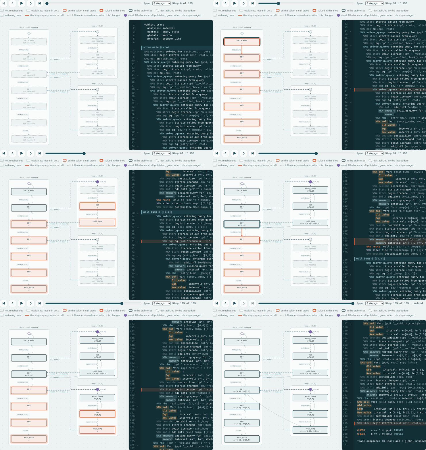
Proof architecture
Inside the boundary drawn in the previous section, soundness is a chain of set inclusions. Start with the stores reached by source executions at one program point. The stores are covered by activation traces, then by context-indexed collecting sets, and finally by the solved abstract states. Each link is a theorem of its own. The analysis may lose precision at every link, but it may not lose a store. One last step turns the final set into the verdict you see. Below, the chain is drawn for n at pp0, the if (n < 2) of this program:
fun f(n) {
  if (n < 2) {
    return 1;
  }
  r = f(n - 1);
  return n * r;
}

fun main() {
  x = f(2);
}
main calls f(2), which calls f(1), so two runs
reach pp0: one with n = 2 and one with n = 1.
Stores a run of pstep has when it is about to test n < 2.
source_reaches_node_collect
the simulation matches each source run to an activation trace in valid_activation_trace that ends at pp0 with the same store
node_collect pp0
The sink_store of every local
trace the graph admits whose
sink_node is pp0,
with the activation each belonged to forgotten.
activation_collect_unit_eq_node_collect
entry_state_node_collect_eq_Union_of_terminates
activation_collect pp0 cThe same activation traces, grouped by the contexts their activation was analyzed under; the key is obtained from the trace, which may belong to multiple contexts.
activation_collect_dg_sound
given a post-solution and a sound specification, every trace step stays inside
γ; the induction itself is
activation_collect_sound,
which bounds the collection by any cover meeting five local obligations
γ(σ (pp0, c))
A post-solution whenever the solve terminates
(the vendored partial_post_solution, with termination discharged by
solve_dom_of_solve_c),
read back as the result the analyzer reports
(gamma_reader_eq_lookup).
run_voblint_check_sound
a verdict at pp0 is decided only when it holds in every store that rung 4 admits, and rung 1 lies inside rung 4, so a PROVED verdict holds in every run that reaches the point. The inclusions between these sets justify the final verdict.fun_route_result_node_sound
without context, and into
entry_state_lookup_sound_of_terminates
with entry-state contexts;
run_voblint_source_sound, the first
flagship theorem below, adds link 1. On the executable side, one more step transports the solver's
association-list states to the function-valued states these sets are stated over.
The chain connects real runs to the verdicts, and the displayed argument uses two theorems and three obligations the analyzer has to discharge. Remove one to see which answers stop being covered.
All five pillars stand, so every store a real run has reaches a verdict that covers it. Click a pillar to remove it.
csim_step, is proved once, for the compiler. It also needs the other half of the simulation, which carries a source run into a valid activation trace. Pillar 2, sound_local_spec, is what every selectable analysis must prove about its transfers, and pillar 5, classify_proved, is what its check classifier must satisfy. A numeric domain proves neither by hand. It certifies one bundle of value operations once, in sound_nonrelational_ops, and both pillars follow from that certificate. The order analysis proves pillar 2 directly (order_spec_sound). Pillar 3, routing_adequate, is discharged by each context policy. Pillar 4 connects to the vendored solver's own theorem, which promises a post-solution only for a solve that terminates. The analyzer runs the executable solver, which answers only where the solve terminates, so an answer discharges that condition (solve_c_run) and no flagship theorem below takes it as a premise.
The diagram omits initial-state coverage and the correspondence of executable states to the transfers and routes used in the theorems. For a numeric domain, the transfer half of the second also follows from the bundle. The executable transfer and the one the proofs use are built from the same operations, and tf_st_for_commute shows that they agree on every live state. The failures shown are what the obligations rule out; they are not bugs anyone has found in Voblint.
Stating the soundness theorem precisely exposed design constraints on the analyzer. The first two below are necessity results. Weakening the condition while keeping the others admits an unsound claim. These results establish necessity for the exhibited conditions. They do not establish necessity for every premise in the development. The third is an executable witness that the implemented equation system obeys another constraint the proof exposed.
Read a callee's result at the callee's context
Tempting When a call returns, read the callee's exit at the caller's own context, since that is the context the caller is in.
Fails on The program fun f(n) { return n; } with a = f(1); b = f(5);, where the context of f is the entry value of n. A claim that reads the result that way meets every other obligation, yet covers no store after the first call, although a run gets there. The analysis would call b = f(5) unreachable.
So The return obligation reads the callee's exit at the context the call entered.
return_at_caller_context_unsound
Every call needs a context
Tempting Let a context policy decline some calls, for instance ones it cannot classify. Every call it does classify is still handled soundly.
Fails on The same program, with a policy that admits no context at all. The claim meets the initial, edge, call, and return obligations. After the call, the caller resumes in its own context, where the claim is empty. The reached store therefore lies outside the claim.
So The coverage contract requires totality. Every call the claim covers is admitted at some context.
total_dropped_unsound
Choose the context and publish the seed from the same state
Tempting Pick the callee's context from the caller's state, which is at hand, and publish the entered state the analysis computes for the callee.
Fails on A call whose entered state differs from the caller's. Here the caller holds [1,1] and the entered state is [7,7]. The seed must land at the key of [7,7]; under the caller's key it would describe an activation it does not belong to.
So The call program routes and publishes with the same entered value, and reads the callee's exit at that same key.
w0_seed_at_entered_frame
w0_seed_at_entered_frame and w0_no_seed_at_caller_frame), so it shows the implementation follows the rule, not that every alternative fails.UNKNOWN at every check satisfies the soundness statement (unknown_everywhere_sound), while one that answers PROVED everywhere violates it (proved_everywhere_unsound). The non-vacuity witnesses establish that concrete theorem instances produce definite verdicts (nv_check_proved_sound).1 for the class 1+2ℤ modulo 2 violates the statement that the shipped congruence remainder satisfies, at −5 (prefix_congruence_mod_unsound). Goblint's regression test samples one program; the obligation covers every operand. The obligation is machine-checked. The upstream behavior is documented here without rerunning Goblint.enter returns multiple alternatives, each pair of caller continuation and callee entry has to cover the run together. Covering the caller store with one pair and the entered store with another lets the combined result exclude the run's real value (unpaired_entry_cover_unsound).keyed_multiwrite_buffered_terminates). That the unbuffered system does not terminate is expected, but neither proved nor evaluated.Formal results
The following theorems concern run_voblint, the function called by the browser analyzer. They establish source coverage and report properties. The proof chain is the argument; this section gives the exact statements it ends in, for readers who want to audit them. Select one to see what it assumes and what it proves.
| Symbol | Reads as | In the theories |
|---|---|---|
| γ a | gamma of a | gamma |
| ⟦e⟧e s | the value of e in s | aval |
| ⟦e⟧♯ d | the abstract value of e in d | aval_abs |
| ⟦a⟧♯c | the abstract transfer of action a in component c | abs_step |
| γ d | the stores the abstract state d represents | gamma_S |
| 𝒢,Π ⊢ c →p c' / 𝒢,Π ⊢ c →p* c' | c steps to c′ | pstep psteps |
| 𝒢,g ⊢ c →c c' / 𝒢,g ⊢ c →c* c' | c steps to c′ in g | cstep csteps |
| Π,g,p ⊢ c ≈ c' | c is matched with c′ | csim |
| p,s0 ⊢ c ⊳ v | from s₀, c is observed at node v in p | at_node |
| skip♯ S / assign♯ S / special♯ S / branch♯ S / body♯ S / return♯ S / event♯ S | the op transfer of analysis S | dgs_skip dgs_assign dgs_special dgs_branch dgs_body dgs_return dgs_event |
| enter♯ S / combine_env♯ S / combine_assign♯ S | the call-boundary transfers of analysis S | dgs_enter dgs_combine_env dgs_combine_assign |
| combine♯ 𝒢 dst q r | the abstract return of r into q | combine_collect_abs |
| context♯ | the computed callee context | route |
| a ∇ b / a Δ b | a widened by b, a narrowed by b | widen narrow |
| 𝒢 | the global-variable classifier | declared_global |
𝒯𝒢,g,SWithin activation_coverage, the fixed parameters are omitted: 𝒯 | the valid activation traces of g from S | valid_activation_trace |
𝒞𝒢,g,S vWithin activation_coverage, the fixed parameters are omitted: 𝒞 v | the stores collected at v | node_collect |
𝒜𝒢,adm,c₀,g,S v cWithin activation_coverage, the fixed parameters are omitted: 𝒜 v c | the stores collected at v in context c | activation_collect |
| ℛres v | the stores report res describes at v | report_sem |
| 𝒱res v | the stores the verdicts of res at v hold in | verdict_stores |
Each name links to its declaration. The README's notation table also gives the meaning of every symbol and the proof-local shorthands.
run_voblint_source_sound in the formalization ↗srun_voblint … = Analysed resv: (residual, s, frs) ⊳ vat every such v: s ∈ node_collect vs ∈ ℛres vs ∈ 𝒱res vHover or focus a premise or conclusion for what it says exactly.
Run the program from any initial store whose globals start at zero, and stop
anywhere. Suppose the analyzer returns Analysed res. At every observation node, the reached store belongs to the collecting semantics and is described by a reported state. Every definite verdict at that node holds for the store. Termination is not a premise. The analyzer runs the executable solver,
and an answer means that solve finished.
The theorem also says where the run is observed, written
p, s0 ⊢ (residual, s, frs) ⊳ v, and its guarantees hold at every
such node. The residual command alone does not determine the node, because in if (b) { x = 1; } else { x = 1; } both
branches leave the same command behind at different nodes. The relation therefore
reads the run through the program's annotated syntax, which labels every
statement with the nodes the compiler emits for it and compiles to the same graph.
The annotated command at which the run stopped names v, and the
compiler's simulation relates the source state to it. A configuration
reachable along two paths can be observed at two nodes. The annotated syntax is used only
in the proof, and the analyzer runs the program as written.
theorem run_voblint_source_sound:
  assumes "s0 ∈ cinit_stores (declared_global p)"
      and "declared_global p, prog_table p
             ⊢ (main_body (prog_table p), s0, []) →p* (residual, s, frs)"
      and "run_voblint config p = Analysed res"
  shows "(∃v. p, s0 ⊢ (residual, s, frs) ⊳ v)
       ∧ (∀v. p, s0 ⊢ (residual, s, frs) ⊳ v ⟶
                s ∈ 𝒞declared_global p,prog_cfg p,cinit_stores (declared_global p) v
              ∧ s ∈ ℛres v
              ∧ s ∈ 𝒱res v)"
run_voblint_check_sound in the formalization ↗snext: __voblint_check(e)run_voblint … = Analysed rese is listed where s isit is not DEADPROVED ⇒ e true in s; REFUTED ⇒ falseHover or focus a premise or conclusion for what it says exactly.
A run about to execute __voblint_check(e) finds a check for
e in the result, listed at a node its store reaches. That check is not
DEAD; if it says PROVED, e is true in the store, and if it says
REFUTED, e is false. The theorem locates the node. Two identical
procedure bodies list their checks separately.
theorem run_voblint_check_sound:
  assumes "s0 ∈ cinit_stores (declared_global p)"
      and "declared_global p, prog_table p
             ⊢ (main_body (prog_table p), s0, []) →p* (residual, s, frs)"
      and "next_check residual = Some (l, e)"
      and "run_voblint config p = Analysed res"
  shows "∃c ∈ set (report_checks res). check_label c = l ∧ check_exp c = e
           ∧ s ∈ 𝒞declared_global p,prog_cfg p,cinit_stores (declared_global p) (check_point c)
           ∧ check_verdict c ≠ Dead
           ∧ (check_verdict c = Decided Check_Proved ⟶ truthy (⟦e⟧e s))
           ∧ (check_verdict c = Decided Check_Refuted ⟶ ¬ truthy (⟦e⟧e s))"
run_voblint_dead_check_unreached in the formalization ↗run_voblint … = Analysed rescheck chk is listedits verdict is DEADnode_collect at its node = ∅Hover or focus a premise or conclusion for what it says exactly.
If a listed check is DEAD, the collecting semantics at its node is empty. No run of the program, starting with its globals at zero, ever reaches that node of the compiled graph. A DEAD check means every state the report holds at its node is ⊥, so the report's semantics there is empty, and the collecting semantics lies inside it.
corollary run_voblint_dead_check_unreached:
  assumes "run_voblint config p = Analysed res"
      and "chk ∈ set (report_checks res)"
      and "check_verdict chk = Dead"
  shows "𝒞declared_global p,prog_cfg p,cinit_stores (declared_global p) (check_point chk) = {}"
run_voblint_arithmetic_safe in the formalization ↗run_voblint … = Analysed ress ∈ node_collect vno diagnostic listed at vv is 0 in sHover or focus a premise or conclusion for what it says exactly.
At a node with no arithmetic diagnostic, every store the program reaches is
arithmetically safe. This property covers the expressions on the edges leaving it, including a
call's arguments. The corollary run_voblint_arithmetic_intra_safe states
it for intra edges. Every divisor in an expression on such an edge evaluates to a
non-zero value.
theorem run_voblint_arithmetic_safe:
  assumes "run_voblint config p = Analysed res"
      and "s ∈ 𝒞declared_global p,prog_cfg p,cinit_stores (declared_global p) v"
      and "∀d ∈ set (report_diagnostics res). diagnostic_point d ≠ v"
  shows "arithmetic_safe_at (prog_cfg p) v s"
run_voblint_check_sites in the formalization ↗run_voblint … = Analysed resHover or focus a premise or conclusion for what it says exactly.
Whatever the configuration, the result lists exactly one check per check in the compiled graph, at that check's node, with its label and condition, in graph order. No check is silently dropped. The label is the check's source position. Writing it in the parser and printing it in the renderer happen outside the proof.
corollary run_voblint_check_sites:
  assumes "run_voblint config p = Analysed res"
  shows "map (λchk. (check_point chk, check_label chk, check_exp chk)) (report_checks res)
           = check_sites (prog_cfg p)"
fun main() {
  n = __voblint_nondet_int();
  if (n > 0) {
    q = 10 / n;
    __voblint_check(n >= 1);
  } else {
    if (n > 5) { __voblint_check(n == 0); }
  }
}
Hover a premise or conclusion to see where it lives. Open this program ↗
run_voblint calls the executable solver, a partial function that answers only where the solve terminates, and builds the report from that answer (solve_c_run). Termination is still not proved in general. Where the solve does not terminate, the analyzer does not answer and no theorem applies. The guarantees are partial correctness.A verdict on the screen rests on a stack of claims. The zoom below starts at the verdict for the counting loop's check and follows one real run, the one that leaves the loop with i = 5, down to the arithmetic lemma it depends on and the proof that Isabelle checks.
What you see
i = 0;
while (i < 5) {
  i = i + 1;
}
__voblint_check(i == 5);   ✓ PROVED
Read as: every run that reaches this line has i = 5.
The flagship theorem
check_verdict c = Decided Check_Proved ⟶ truthy (⟦e⟧e s)
For every store s a source run has when it is about to run the check,
a listed check for i == 5 sits at a node s reaches, and
PROVED there makes i == 5 true in s.
Why the verdict may say PROVED
classify c d = Check_Proved ⟹ s ∈ γ d ⟹ truthy (⟦c⟧e s)
The analysis says PROVED only when every store its state d describes
satisfies the check. At the check, d is i ∈ [5, 5]: one
value, and it is 5. The classifier is shared across domains. It is
built from the two comparison queries of Interval's operation bundle, and this
lemma is proved once for every domain that supplies such a bundle.
Run coverage by d
𝒞𝒢,prog_cfg p,cinit_stores 𝒢 v ⊆ γ (state_at 𝒢 p v)
Every store the collecting semantics reaches at the check's node lies in the
concretization of the result there. Our run's store, i = 5, is in
γ([5, 5]).
Coverage of graph nodes
activation_collect 𝒢 adm c₀ g S v c ⊆ cover v c
By induction along the run's trace E → H → B → H → … → X: if one
store is covered by the solver's value at its node, the next store is covered at
the next node. The solver's post-solution supplies the value, each edge's
transfer supplies the step.
One step: the edge i := i + 1
s ∈ γ σ ⟹ s(x := ⟦a⟧e s) ∈ γ (assign x a σ)
On its last pass the run is at B with i = 4, inside
σ(B) = [0, 4]. The transfer contract requires that the
assignment must cover the store after the step, i = 5. No numeric domain
writes its assignment transfer by hand. The transfer is built from the domain's evaluator,
and this lemma is proved once for every certified bundle.
The right-hand side i + 1
s ∈ γ σ ⟹ ⟦e⟧e s ∈ γ (⟦e⟧♯ σ)
If every variable's value is covered by the abstract state, evaluating the
expression abstractly covers evaluating it concretely: 4 + 1 = 5
lies in γ([0, 4] + [1, 1]).
One operator: interval addition
i ∈ γ a ⟹ j ∈ γ b ⟹ i + j ∈ γ (a + b)
With i = 4 ∈ γ [0, 4] and j = 1 ∈ γ [1, 1], the lemma
gives 5 ∈ γ [1, 5]. Everything above rests on lemmas of this size.
What γ is
gamma_ivl (Ivl l u) = {n. l ≤ Fin n ∧ Fin n ≤ u}
Every rung above is an ∈ γ claim, and this is where
γ stops being a symbol. An interval is a pair of
eint
bounds, each MinInf, Fin of an integer, or
PlusInf. So [0, 4] is
Ivl (Fin 0) (Fin 4), and the set it stands for is the
comprehension above: {0, 1, 2, 3, 4}. The chain of definitions ends here. The
integers are HOL's, and the order on eint has three cases.
The bottom: a proof
lemma ivl_plus_sound:
  assumes "i ∈ gamma_ivl a" "j ∈ gamma_ivl b"
  shows "i + j ∈ gamma_ivl (a + b)"
proof (cases a; cases b)
  …
  show "i + j ∈ gamma_ivl (a + b)"
    unfolding ‹a = Ivl l1 u1› ‹b = Ivl l2 u2›
    using bnds normalize_ivl_def
    by (cases l1; cases l2; cases u1; cases u2) auto
qed
A three-way case split on each of the four bounds (−∞, a number, +∞), every
case closed by auto. Isabelle's kernel replays every inference.
i = i + 1, so the operator lemma there
is the one for addition, such as congruence_plus_sound in the congruence
domain. Congruence, Sign and Parity answer UNKNOWN on this check, so the zoom has no
PROVED to start from in those.
The zoom followed one path. The development has layers for semantics, compilation, abstract domains, equations, and solving. Stations on one line belong to the same layer and are listed in reading order. Only the interchanges claim that one result uses another. All five lines reach the result line, which ends at the verdicts you see. Hover over a station to see its theory, and click it to open the theory.
activation_collect_dg_sound Voblint_Framework.Routed_Context
This theorem connects semantics, framework, and solver. It assumes a post-solution of the routed equations, a sound specification, and the context-policy obligations. Every trace-reached store lies in γ of the solved value.
Stations are real definitions, theorems and the obligations an analysis discharges;
wide markers are interchanges, where one result consumes the others that meet there. Being next
to each other on a line says only that two stations belong to the same layer. The map
follows the session structure. The semantics line lives in Voblint_VIMP
and Voblint_CFG, the compiler in Voblint_Compile, the domain
line in Voblint_Nonrelational, for its executable refinement
Voblint_Exec, and, for its branch,
Voblint_Analysis_Relational, the framework line in
Voblint_Framework, the solver in the
vendored TD session, Voblint_Solver and
Voblint_Exec, and the result line in Voblint_Routing,
Voblint_Result and Voblint_CLI.
All three terminals are proved from one hub,
run_voblint_covers,
which says that the report's semantics at a node of the graph contains every store the
collecting semantics has there.
The semantics line therefore continues into the central interchange. DEAD and SAFE are
stated over node_collect
too. The theorem
run_voblint_source_sound
adds the source run. PROVED is the only terminal stated at a source run. DEAD skips it on
purpose. The bridge runs forwards, placing each run at the nodes it is observed at (p, s0 ⊢ … ⊳ v), so it
cannot be read backwards into “no run reaches this node”. That claim is proved
forwards from the hub, at every collected store.
The result line splits once per kind of context policy. Policies that
compute a context from the call alone go through
fun_route_result_node_sound;
entry-state contexts, obtained from the solved result, go through
entry_state_policy_of_terminates.
A second endpoint,
run_voblint_spine,
keeps the contexts that run_voblint_source_sound erases. Per
policy, it places a run's store in the collecting semantics of one context
its activation trace carries. It is an interchange of the compiler and
result lines like the headline, and both branch from
run_voblint_contexts,
where the two routes rejoin.
Inside the development
The proof chain follows the main soundness results. The interactive proof map lets you explore the declarations around them, from the source semantics to the domain instances and the executable analyzer.
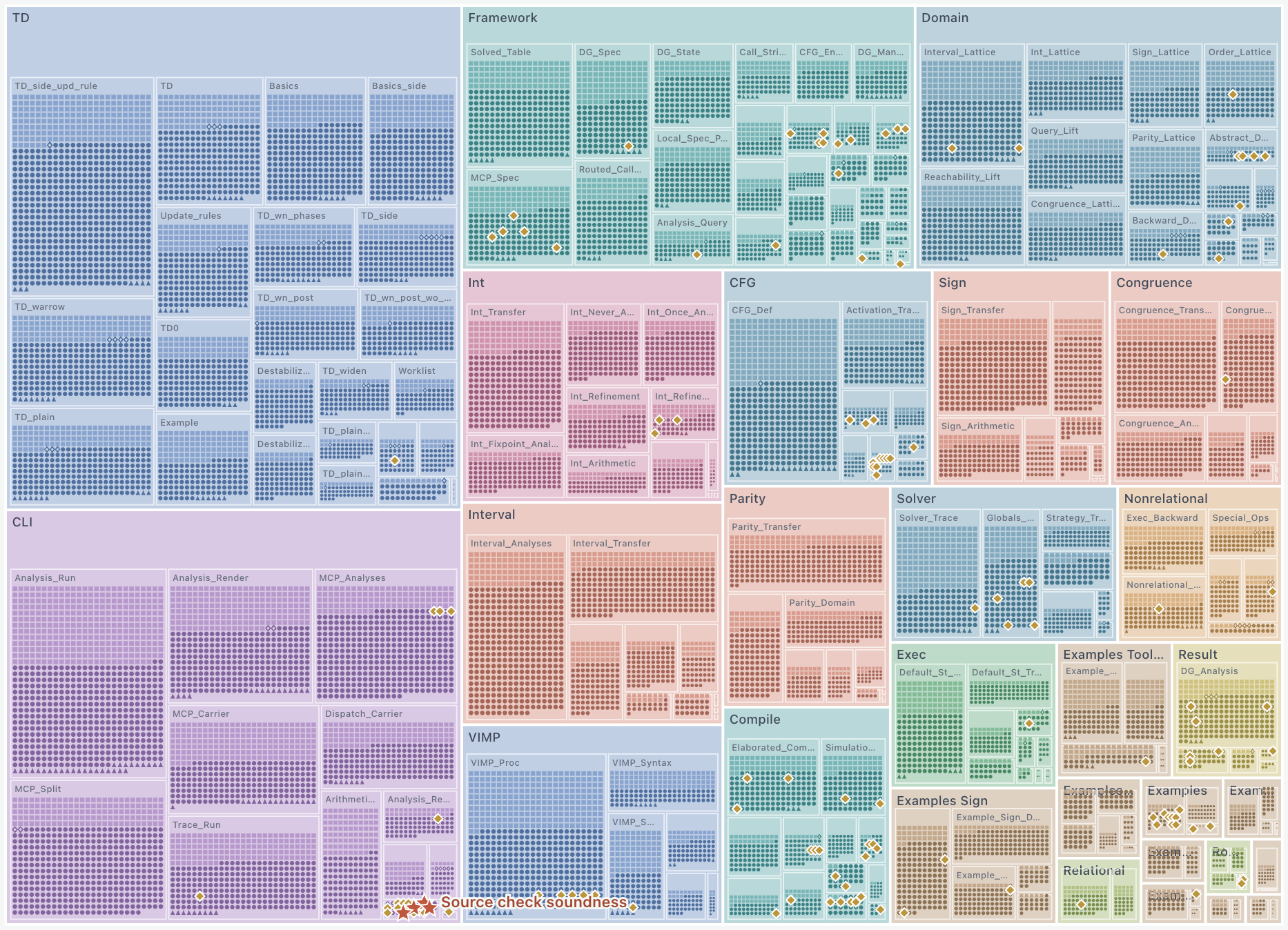
Each small mark is an exported fact, constant, type or locale, including automatically generated declarations. The treemap groups them by session and theory; block area follows the number of entities. Colors match the dependency layers in the strata figure below. Gold diamonds mark facts cited in the thesis, and red stars mark selected source-level soundness results.
Switch to the corpus wheel to follow each theory’s declarations in radial streaks. Pinch to reveal more detail, use two-finger scrolling to pan, or search for a name. Click a mark to open its Isabelle documentation. The connecting lines show references in statements and specifications; they do not record which lemmas a proof uses.
Goblint correspondence
Voblint follows the architecture of Goblint, a static analyzer for C programs. Voblint analyzes VIMP instead, a small imperative language with integer variables, globals and recursive procedures (see what it leaves out). What we claim is a simplified, machine-checked semantic model of Goblint's interprocedural, context-sensitive architecture, not a model of its implementation. The vocabulary of locals, globals and side effects follows the FM 2026 tutorial on mixed flow-sensitivity by Goblint's authors.
EvalInt of its condition. Only EvalInt exists, answers are not cached, and a combined analysis reads and publishes no globals of its own.
One row of the table deserves more than a line. Five of the six analyses keep a pointwise state, one abstract value per variable, so it is fair to ask whether the framework works only for that shape. The sixth, the order analysis, shows that it does not. The order domain's carrier is a set of known pairs x ≤ y, and it contains no vname ⇒ 'a anywhere. Rel_Order_Domain interprets analysis_contract with this carrier without any change to the framework, and Rel_Order_Local runs the same carrier inside the combined state, next to the other analyses. There it uses the same interface as every selectable analysis. It supplies a local_spec and proves it sound (order_spec_sound), the interface the five pointwise analyses reach through their certified operation bundles. It answers comparisons from the pairs it records, and at an assignment it asks the other analyses how the new value compares with each variable. The analysis computes no transitive closure, and calls enter and return with no facts. Together with Interval, it proves checks that neither analysis proves alone (an example).
Cost
Most programs in the regression corpus are quick to analyze. The median one solves in a few milliseconds natively. A proof says nothing about speed, though, and some settings are expensive. The numbers here come from the recorded measurement, on one machine.
Contexts are where the cost goes. With entry-state contexts a
recursive procedure gets one context for every abstract argument it is entered with.
Under the interval domain, which distinguishes individual numbers, h(n) counting
down from n therefore keeps n + 1 copies of h
apart. That copy count drives the run time.
A CPU profile of such a run spends much of its own time in the generated code's list
lookups, which compare nodes and contexts one at a time.
The playground runs the same generated code compiled to WebAssembly. It is slower than the native command line.
The profiling page documents the measurements and methods. It includes results for each domain and context policy across the corpus, scaling curves, and an interactive CPU profile. These measurements do not establish bounds for arbitrary programs. Whether the solver finishes at all is a premise checked per program, as the next section explains.
Limitations
Voblint's soundness theorems hold for a small language under a fixed set of assumptions. This section describes what lies outside them.
Goblint analyzes C. Voblint analyzes VIMP, a language small enough that its semantics could be written down and every analysis step proved against it. Hover a region to see what VIMP leaves out.
Hover or focus a region.
Every soundness guarantee assumes the solve terminates. Proving that in general is out of scope; for intervals, the join-based rules give no answer within a time limit on some programs, and so do entry-state contexts. We expect these solves to diverge, but a timeout does not prove it.
A program failing wf_program_compile_input_exec
receives Malformed_Program and is never analysed. The
Analysed res premise excludes rejected programs from the theorem.
There is no completeness claim. A correct result may still say UNKNOWN for a check that holds.
REFUTED says the check fails in every run that reaches it, not that any run does. An error diagnostic likewise does not prove the point is reachable.
The parser is generated from one grammar and tested. Isabelle's code generator, the OCaml compiler, wasm and your browser are trusted. Source positions, badges and graph drawings (OCaml rendering, this page) are unverified.
Voblint models Goblint's design, and no theorem here speaks about Goblint's OCaml implementation.
The generated OCaml is slow. The purely functional implementation uses association lists for most maps and sets, with red-black trees in a few components. These representations simplify the proofs.
x != 5Goblint's exclusion sets are absent. Over unbounded integers, joining 5 and 7 has no least upper bound among them, so exclusion sets cannot form the lattice these domains require.
The analyzer that runs is a small part of the project. Most of the work went into definitions of what a program means and into proofs that every step of the analysis respects them.
Isabelle lines per area
Regression corpus by what the program does
precision: the answer is fixed by the source and the analysis must find it.
soundness: runs disagree, so UNKNOWN is the only right answer.
known imprecision: fixed, but out of the abstraction's reach.
What the theories contain
one square = 10 statements or declarations; hover a kind to pick it out
Counted by keyword, the way pixi run theory-stats --view kinds counts them. A lemma or definition inside a locale counts once, and
fun and primrec are both recursive functions.
When it was written
One square per day, darker for more commits, counted by author date over the whole history of the repository when the site was built.
pixi run theory-stats over src. The
solver berg counts only the vendored theories Voblint's sessions import, directly or
through each other; the rest of that development verifies solver variants Voblint does
not use. The exported OCaml module and the handwritten OCaml under cli are
plain line counts. Counted when the site
was built.
The iceberg shows the size of the development; this figure shows its structure. Every Isabelle session is a rock layer, placed just above the highest session it builds on, from the logic at the bottom to the examples at the surface. Hover over a session, and the layers it rests on light up. A layer's thickness grows with its line count, so the core sample also shows where most of the material is.
The CLI and browser expose all six analyses: Sign, Interval, Parity, Congruence, Int and relational Order. Order sits lower because it supplies its local specification directly, without the non-relational builder. Hover over CLI to see the dependencies of their shared entry point.
Core sample
Voblint_CLI
Includes Sign, Interval, Parity, Congruence, Int and Relational.
run_voblint exposes Sign, Interval, Parity, Congruence, Int and relational Order to the CLI and browser. This session assembles their cooperating local specifications and proves the source-level soundness results.
Hover a layer to highlight its session dependencies. Click to open the session.
ROOTS lies one layer above the highest session it rests on,
where resting on means its ROOT parent, a session its ROOT lists, or
a session one of its theories imports. The site build reads all three from the sources
(scripts/session_graph.py), so the layers follow the development. A layer shows
order, rather than every contact. Hovering a session outlines what it rests on directly in bold and
everything below that, reached through those, in a lighter dotted line. The example sessions
are drawn together at the surface. Lines are counted per ROOT directory with the
scanner behind pixi run theory-stats:
59,477 in src plus
30,560 across the
26 theory files in the vendored solver's directory,
of which Voblint's imports reach 7 theories and
9,533 lines. A layer is 22 px plus a height
proportional to its lines; sessions sharing a layer are as wide as their share of its lines,
but at least 104 px so every name fits. The bedrock is not to scale, and lemmas count
the proofs the scanner finds.
Related work
Goblint is developed at TUM and the University of Tartu. The groups below run from the oldest ideas this page builds on to the solver proofs it imports. If you read one, read the FM 2026 tutorial on mixed flow-sensitivity, whose vocabulary this page uses. The full list, theses included, is on Goblint's publication page, and the analyzer itself is described in its documentation.
Hover or focus a dot to see the paper; click it to jump to its entry.
export_code, which turns the proved definitions into the OCaml you run.
valid_activation_trace trace set.
Documentation and tools
Start from the certified pipeline theory for the compact theorem-level view, or browse the generated Isabelle documentation for the complete development.
Voblint.thy, the downstream entry point that presents
the certified pipeline and links its major layers and flagship theorems.